Hãy viết lại bài viết dài kèm hashtag về việc đánh giá sản phẩm và mua ngay tại Queen Mobile bằng tiếng VIệt: How to use the VLOOKUP function

Mua ngay sản phẩm tại Việt Nam:
QUEEN MOBILE chuyên cung cấp điện thoại Iphone, máy tính bảng Ipad, đồng hồ Smartwatch và các phụ kiện APPLE và các giải pháp điện tử và nhà thông minh. Queen Mobile rất hân hạnh được phục vụ quý khách….
_____________________________________________________
Mua #Điện_thoại #iphone #ipad #macbook #samsung #xiaomi #poco #oppo #snapdragon giá tốt, hãy ghé [𝑸𝑼𝑬𝑬𝑵 𝑴𝑶𝑩𝑰𝑳𝑬] ✿ 149 Hòa Bình, phường Hiệp Tân, quận Tân Phú, TP HCM
✿ 402B, Hai Bà Trưng, P Tân Định, Q 1, HCM
✿ 287 đường 3/2 P 10, Q 10, HCM
Hotline (miễn phí) 19003190
Thu cũ đổi mới
Rẻ hơn hoàn tiền
Góp 0%

Thời gian làm việc: 9h – 21h.

KẾT LUẬN

Hãy viết đoạn tóm tắt về nội dung bằng tiếng việt kích thích người mua: How to use the VLOOKUP function

There are numerous ways to search Google Sheets, and the find and replace feature is among these techniques. It works well with unstructured data and helps you locate values. When you’re working with a large dataset, you’ll spend more time remembering the exact order of characters. If you don’t, you’ll manually scan your spreadsheet.

Use the VLOOKUP search function on your new Chromebook or laptop to customize your search, and data retrieval is instant. The formula finds data using a combination of focus keys and defined ranges and then consolidates it into your preferred cells. You’ll bring together important data without copying and pasting. Here’s how to use this time-saving function.

What is VLOOKUP, and what does it do?

Vertical lookup, or VLOOKUP, is a search function that finds a value in a column and its correspondents in the same row.

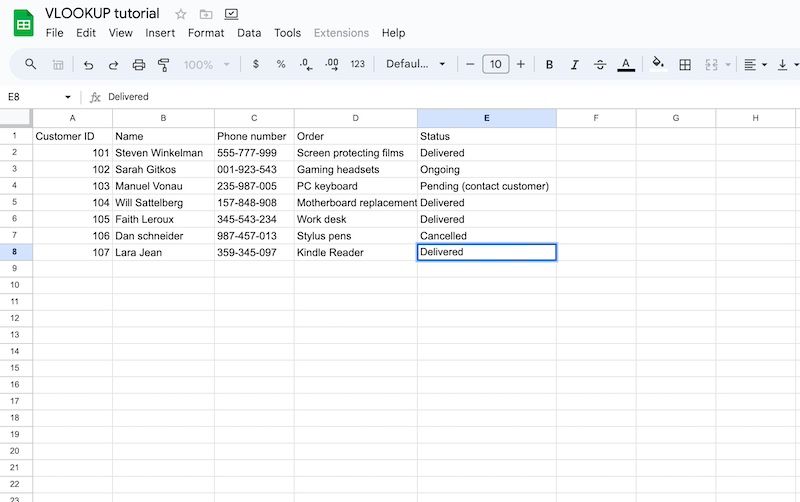
Let’s say you want to find a customer’s phone number in a spreadsheet but don’t know the exact digits. However, you know it’s under the Phone number or contact information column. Rather than scrolling through the list, use a formula to pull up the results.

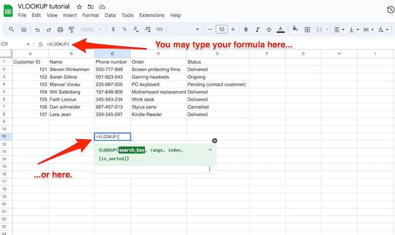
Start the formula with the =VLOOKUP formula in the cell where Sheets should display the result. Alternatively, type it in the formula field above the spreadsheet. Then add the following parameters, breaking each one with a comma.

Search_key

This parameter represents the value VLOOKUP should search for in the first column of the dataset range. Insert it as shown below, replacing search_key with a specific value. Using our previous customer example, their phone number, ID number, or other identifiers can be your search key.

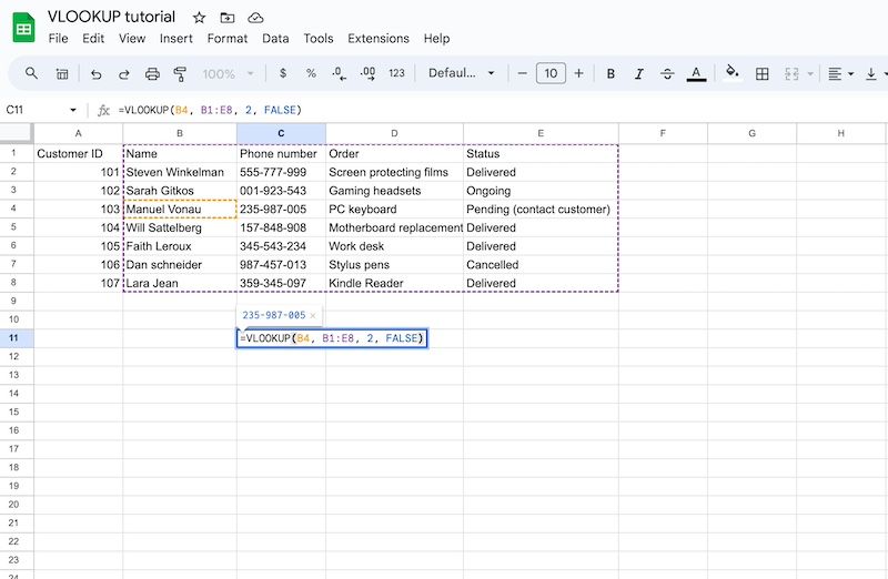
If you use a name or phrase, put quotes around the name so that Sheets looks for it specifically. For example, “Tom Bradley”. Alternatively, reference the cell number if you recall it. If the name Tom Bradley is in cell B4, type B4 in the formula as your search key.

=VLOOKUP(search_key, …)

Range

It’s the area of cells where you want Sheets to limit the search. For example, B1:C8. You can also highlight all values in the spreadsheet or click and drag across cells to define them in the formula.

=VLOOKUP(search_key, range…)

Index

Sheets now knows where to look for a search value and what range to search, but what information do you want it to bring back? Index is the return value column. It’s where the exact value you’re looking for resides. Think of it as numbering or counting the cell ranges you defined in the formula.

If the range you defined is C1:G5, that’s five columns you’re instructing Sheets to comb through. If the exact data you’re looking for is in the C column, your index is 1. If it’s in the F column, the index is 4.

=VLOOKUP(search_key, range, index, …)

Is_sorted

This parameter is optional, but for most datasets, indicate it as FALSE. It ensures that VLOOKUP returns an exact match and produces an error message if it doesn’t find the information you’re looking for. If you leave it unspecified or indicate it as TRUE, Sheets allows for an approximate match, grabbing a nearby value to return.

Use it for organized values in ascending order or to find the next-highest price, the closest ID number, or other variations.

=VLOOKUP(search_key, range, index, is_sorted)

How to use VLOOKUP on Google Sheets

VLOOKUP acts as a search box and returns customized results from a large dataset. The formula works if you apply it to your spreadsheets on the mobile or web apps. Use the web version on a computer when possible as it provides a wider layout to work easily.

For this walkthrough, let’s find the phone number for our customer, Manuel Vonau. Manuel ordered a PC keyboard. We need to contact him because there was an issue with the order, causing a delay. We’ll use the VLOOKUP function to find his phone number in the store database.

Use VLOOKUP on the Google Sheets web app

1. From a PC browser, visit docs.google.com/spreadsheets and open a spreadsheet.
2. Click the cell where you want Sheets to apply the formula and display the results.
3. Type =VLOOKUP in the cell or the formula field above the spreadsheet. Then, enter an open bracket.
   

4. Type your search_key. In this case, the cell number for Manuel’s name is B3. Put a comma afterward.
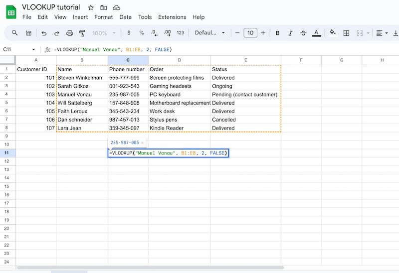
5. Since we’re using Manuel’s name, we’ll put quotes around it. For example, “Manuel Vonau”.
   

6. Enter the cell range Sheets should search for the phone number. For example, B1:E8. Enter a comma afterward.
7. Type the index. Our index is 2 because the phone number is in the second column of our defined range.
8. Set a TRUE parameter if you want Sheets to consider the nearest results. Enter FALSE if you want an exact match. This step is optional.
   

9. Close the formula with a bracket and press Enter or return on your keyboard to run it. Sheets displays the phone number requested in the selected cell.

Use VLOOKUP on the Google Sheets mobile app

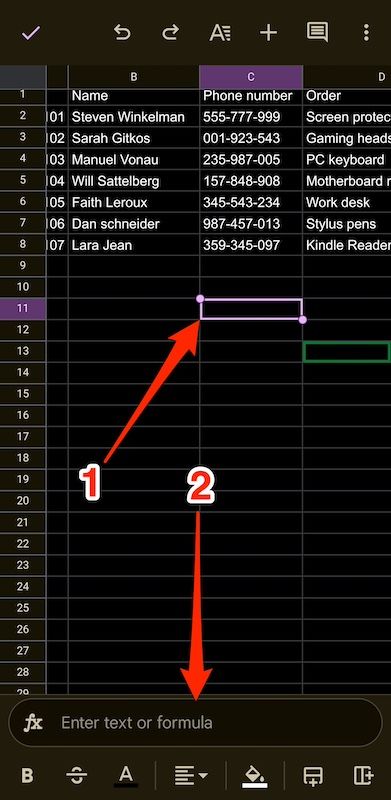
1. Open a spreadsheet and tap the cell where Sheets will display the search result.
2. Tap the text box at the bottom of the screen to start typing the formula.
3. Type =VLOOKUP, then tap VLOOKUP above the text box to place the formula bracket.
   

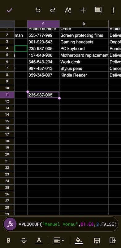
4. Inside the bracket, enter your search_key. In this case, we use “Manuel Vonau”. Add a comma afterward.
5. Type the cell range. We use B1:E8. Enter a comma afterward.
6. Type the index. It’s 2 as the phone number is in the second column of our defined range.
7. Tap the enter button on your keyboard to run the formula. Sheets displays the requested customer phone number.
   

A few tips for using VLOOKUP in Google Sheets

Depending on how often you use VLOOKUP or what role it plays, take note of the following factors:

• Searches must be exact. Make sure collaborators understand that every character they type must be accurate for VLOOKUP to work.
• Replace the error value. VLOOKUP returns #N/A if it doesn’t find results from the search. That’s fine for internal use but may confuse casual users. Use the IFNA() function to replace that return with alternative text, typically “Not Found.”
• Use quotation or question marks as your search_key to look for a specific character, such as “T?” to return the entry starting with a capital T. An asterisk does the same for multiple letters.

VLOOKUP presents a systematic approach to data matching

Now that you’ve created a VLOOKUP solution, explore other Sheets tricks and shortcuts. You can freeze rows or columns so that they move with you as you scroll around your spreadsheet. Another way to organize your spreadsheet is to filter data by color, condition, and values. These features help you navigate your spreadsheets faster and work efficiently. Also, collaborators can use them.